
The combination of time series analysis and Design of Experiments (DOE) is a critical tool for corporate executives and process optimizers trying to enhance operational forecasting in an increasingly data-driven world. This formal method takes advantage of the sequential character of time series data and DOE’s capability for systematic exploration.
This combination improves the accuracy of future operational performance projections. It allows for a more in-depth understanding of prior data trends, laying the groundwork for strategic planning and informed decision-making.
Takeaways
- The integration of Time Series Analysis (TSA) with Design of Experiments (DOE) enhances operational forecasting, offering a robust tool for data-driven decision-making.
- Key components of TSA, including trends, cyclical variations, and seasonal patterns, are essential for understanding and forecasting data over time.
- Incorporating TSA models within DOE provides a systematic approach to examining how variables change over time, affecting outcomes and improving forecasting accuracy.
- This methodological integration across various industries enables organizations to anticipate future trends better, optimizing operational efficiency and strategic planning.
Key Concepts of Time Series Analysis
Time series analysis is a statistical technique that analyzes data points collected over time intervals. This method is instrumental in making predictions based on time, such as stock market projections and weather forecasting. The core components of time series analysis include trends, cyclical variations, random or irregular movements, and seasonal variations. Each element is crucial in understanding and forecasting data patterns over time.
Basic Elements of Time Series Analysis
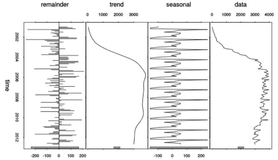
Image Source: Wikimedia Commons
Trend
The trend component reflects the long-term direction in which a data series moves. It indicates whether the series shows a general increase, decrease, or stability over time. Trends are crucial for understanding the overarching movements in the data, such as a consistent rise in e-commerce sales over several years or a gradual decrease in pollution levels due to environmental policies. Many factors, including economic, social, and technological changes, can influence trends.
Cyclical Variations
Cyclical variations, unlike seasonal variations, do not have a fixed period. They are often tied to economic cycles and can last for more than a year, sometimes spanning several years. These cycles are characterized by economic expansions and recessions, reflecting periods of growth followed by slowdowns. Identifying cyclical variations can help businesses and policymakers make informed decisions by anticipating changes in economic conditions.
Seasonal Variations
Seasonal variations are predictable and recurring patterns observed within specific time intervals, such as days, weeks, months, or quarters. This component is driven by seasonal factors, like weather changes, holidays, and school cycles, affecting consumer behavior, sales, and production. For example, retail businesses often experience higher sales during the holiday season, while energy consumption may peak during the summer and winter due to heating and cooling needs.
Random or Irregular Movements
Random or irregular movements represent the unpredictable fluctuations in a time series. These movements are caused by unforeseen or random events such as natural disasters, strikes, or sudden changes in market conditions. Identifying and understanding these irregularities are essential for accurate forecasting and analysis, as they can significantly impact the overall trend and seasonal patterns.
The interplay of these components within a time series provides a comprehensive view of the data’s behavior over time. Organizations can better predict future trends, adapt strategies, and make informed decisions by analyzing these elements. Techniques such as exploratory analysis, curve fitting, and forecasting leverage these components to extract meaningful insights from time series data.
For instance, exploratory analysis decomposes a series into essential elements, allowing analysts to identify and explain underlying patterns and causes. On the other hand, curve fitting and forecasting enable predictions of future values based on historical patterns, offering valuable insights for planning and strategy development.
Time series analysis, focusing on trends, cyclical and seasonal variations, and random movements, plays a pivotal role in various domains, from finance and economics to environmental studies and healthcare.
Time Series Models
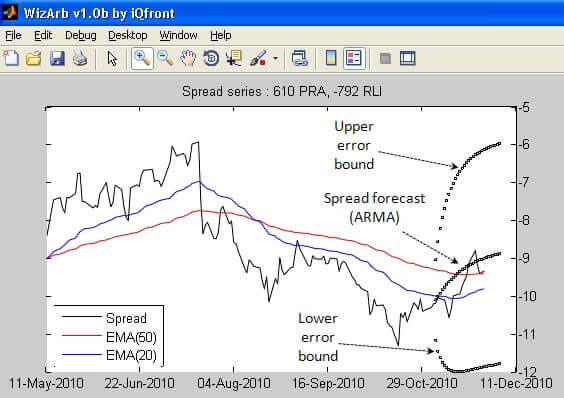
Image Source: Wikipedia
Integrating time series models within the Design of Experiments (DOE) framework can significantly enhance operational forecasting by leveraging the temporal dynamics of data. Let’s explore how each time series model can be incorporated into DOE, providing examples for clearer understanding.
Autoregression Model (AR)
The Autoregression Model (AR) is based on the concept that current observations are correlated with previous ones. In a DOE context, this model can be used to assess the impact of time-dependent interventions on a process or system.
For example, suppose a manufacturing process changes to improve efficiency. In that case, AR models can help quantify the effect of these changes over time, considering the lagged impact of past changes.
Moving Average Model (MA)
The Moving Average Model smooths out short-term fluctuations and highlights longer-term trends or cycles. In DOE, this can be particularly useful for identifying and adjusting for noise in experimental data.
Consider an agricultural experiment aimed at increasing crop yield; an MA model could help isolate the true effect of different fertilizers on yield by smoothing out variations due to weather conditions or other external factors.
Integration (I)
Integration, a component of the ARIMA model, makes non-stationary time series data stationary. This is crucial for accurate modeling and forecasting. Within DOE, integrating time series data can ensure that the analysis is not biased by trends or seasonal effects.
For instance, when evaluating the sales impact of a new marketing campaign, it’s important to differentiate between the campaign’s effectiveness and seasonal sales patterns.
Seasonality (S)
Incorporating seasonality into time series models allows for analyzing patterns that repeat over fixed periods. In DOE, this can be used to plan experiments or interpret results in the context of seasonal variations.
An example could be a retail business testing different staffing levels to optimize customer service during peak and off-peak seasons. By accounting for seasonality, the DOE can more accurately assess the impact of staffing changes.
SARIMA Model
The Seasonal Autoregressive Integrated Moving Average (SARIMA) model combines the aspects of ARIMA with seasonality, making it ideal for forecasting data with seasonal patterns. In DOE, SARIMA models can be used to forecast the outcomes of experiments under different seasonal conditions.
For example, a utility company might use SARIMA to predict the effectiveness of energy-saving measures across different seasons, helping to plan when and where to implement these measures for maximum impact.
Integrating these time series models with DOE offers a robust framework for understanding and predicting the effects of various factors on outcomes over time. This approach allows for the adjustment of models based on historical data and facilitates the design of experiments that can predict future trends, optimize processes, and improve decision-making.
Common Uses of Time Series Models
Image Source: Freepik
Time series models are a cornerstone of data analysis, offering a framework for understanding, predicting, and influencing future trends based on historical data. These models are instrumental across various sectors, providing insights and facilitating decision-making by analyzing data patterns over time. Here’s an expanded look at the common uses of time series models:
Determining Patterns
Time series analysis is pivotal in identifying and understanding recurring patterns within data, such as seasonality and trends. For businesses, recognizing these patterns is crucial for planning and performance evaluation.
For example, retailers can forecast seasonal sales peaks and valleys, allowing them to optimize inventory levels, staff scheduling, and promotional campaigns to match anticipated demand.
Forecasting Future Trends
One of the primary applications of time series models is forecasting future events or trends. This predictive capability is based on the premise that past behaviors and patterns can inform future outcomes. In inventory management, accurate forecasts enable companies to maintain optimal stock levels, reducing overstock and stockouts.
Analysts use time series models in financial markets to predict stock price movements, interest rates, and economic indicators, guiding investment strategies and economic policy.
Detecting Anomalies
Time series models are also adept at identifying anomalies or outliers in data, which can signal errors in data collection, fraudulent activity, or emerging trends. In cybersecurity, time series analysis can detect deviations from standard network traffic patterns, potentially identifying security breaches or attacks.
Healthcare providers use time series analysis to monitor patient data over time, where sudden changes in vital signs can indicate medical emergencies or the development of health conditions.
Industry Applications
- Healthcare: Time series models track the spread of diseases, patient recovery patterns, and the effectiveness of treatment plans. Healthcare professionals can better allocate resources and plan interventions by analyzing the disease’s progression.
- Agriculture: Predicting crop yields becomes more accurate with time series analysis, accounting for seasonal temperatures and rainfall variables. This insight helps farmers decide about planting schedules, irrigation needs, and harvest times.
- Finance: In the financial sector, time series analysis underpins market trend analysis, risk assessment, and algorithmic trading strategies. Analysts predict future market movements to inform investment decisions, while financial institutions assess credit risk and detect fraudulent transactions.
- Cybersecurity: By monitoring network traffic and user behavior over time, time series models can identify unusual patterns that may signify cyber threats or system vulnerabilities, enabling timely responses to potential security incidents.
- Retail: Retailers leverage time series analysis for price optimization, demand forecasting, and customer behavior analysis, enhancing profitability and customer satisfaction.
Integration into Operational Forecasting

Image Source: Freepik
Integrating time series models into operational forecasting involves using historical data to make informed predictions about future trends, demand, and anomalies. This approach enables organizations to anticipate changes, adapt strategies, and optimize operations.
For example, a utility company might use time series forecasting to predict peak electricity demand periods, allowing for more efficient energy production and distribution planning.
The versatility of time series analysis and its predictive power make it an invaluable tool across industries. By harnessing these models’ insights, organizations can understand past trends and anticipate future developments, leading to more informed decision-making and strategic planning.
Methodological Approach to Integration of Time Series Analysis (TSA) and Design of Experiments (DOE) in Forecasting Models

Image Source: Pexels
Integrating Time Series Analysis (TSA) with Design of Experiments (DOE) in forecasting models encompasses a systematic approach that combines the predictive power of TSA with the structured testing capabilities of DOE.
This integration allows for a more nuanced understanding of how variables over time affect outcomes, thus improving forecasting accuracy. Below is a comprehensive, step-by-step guide on effectively integrating these methodologies.
Step 1: Define the Objective
Determine what you aim to forecast and why. This could range from predicting sales volume, and optimizing manufacturing processes to managing supply chain logistics.
Highlight the variables that you believe influence the forecast. These could be seasonal factors, economic indicators, or operational changes.
Step 2: Data Collection
Collect time-series data relevant to the forecasting goal. This includes data points over regular intervals (daily, weekly, monthly).
Plan experiments using DOE principles to systematically vary key variables and observe their effects. This could involve changing one factor at a time or using factorial designs to alter multiple factors simultaneously.
Step 3: Data Preprocessing
Remove anomalies, fill missing values, and ensure data quality. This step is crucial for accurate TSA and DOE analysis.
Segment data should reflect different experimental conditions or periods relevant to the study depending on the objective.
Step 4: Conduct Time Series Analysis
Use TSA to uncover historical data’s underlying patterns, trends, and seasonalities.
Choose appropriate time series models (e.g., ARIMA, SARIMA) based on the data’s characteristics. The selection should consider trends, seasonality, and autocorrelation in the data.
Step 5: Apply Design of Experiments
Apply DOE to investigate how different variables affect the outcome of interest. This could involve controlled experiments or observational studies.
Use statistical methods to analyze the experimental data, identifying significant factors and their interactions.
Step 6: Integrate Findings
Integrate the insights from TSA and DOE. For instance, incorporate the effects of significant variables identified through DOE into the time series model.
Adjust the forecasting model based on DOE outcomes. This might include adding predictors for significant factors or adjusting for seasonality and trends.
Step 7: Forecasting and Validation
Use the refined model to make forecasts. Ensure the model incorporates both the time series analysis findings and the experimental results from DOE.
Validate the forecasts against actual outcomes to assess accuracy. Use evaluation metrics like MAPE (Mean Absolute Percentage Error) or RMSE (Root Mean Square Error).
Step 8: Continuous Improvement
Based on validation results, iteratively refine the model. This could involve collecting more data, conducting additional experiments, or exploring alternative modeling techniques.
Document the process, findings, and model performance. Gather feedback from stakeholders and incorporate it into future iterations.
Considerations
- Data Quality: Ensure high-quality, relevant data for both TSA and DOE. Poor data quality can lead to inaccurate forecasts and misleading experiment results.
- Model Complexity: Balance model complexity with interpretability and practicality. Overly complex models may be more accurate but harder to understand and apply.
- External Factors: Consider external factors not captured in historical data or experiments that could influence forecasts, such as economic shifts or unexpected events.
By following these steps and considerations, organizations can effectively integrate TSA and DOE into their forecasting models, enhancing their ability to make informed decisions and plan for the future more accurately.
Conclusion
Integrating Time Series Analysis (TSA) and Design of Experiments (DOE) into forecasting offers a transformative approach for enhancing operational forecasts and strategic decision-making.
This powerful synergy enables organizations across various industries to anticipate future trends more confidently, facilitating strategic planning and informed decision-making. This integration is critical for achieving operational efficiency and strategic agility in a data-driven world through a structured process from objective definition to model refinement and validation.
At Air Academy Associates, we are dedicated to propelling professionals to new operational efficiency and excellence heights. Our Operational Design of Experiments Course is meticulously crafted to empower you with advanced skills in experimental design, enabling you to unlock significant improvements in product quality, streamline operations, and foster innovation. Join a community of forward-thinking professionals committed to operational mastery. Enroll in our course today!

